|
|
|
|
|
|
|
|
|
|
【Instruction】 |
|
|
|
||
|
|
|
|


In this chapter, we would like to introduce you the basic principles of ladder diagram, in addition, the coding rules of Mnemonic will be introduced as well, it’s essential for the user who use FP-08 as a programming tool. If you are familiar with PLC Ladder Diagram and mnemonic coding rules, you may skip this chapter.
1.1The Operation Principle of Ladder Diagram
Ladder Diagram is a type of graphic language for automatic control systems it had been used for a long period since World War II. Until today, it is the oldest and most popular language for automatic control systems. Originally there are only few basic elements available such as A-contact (Normally ON), B contact (Normally OFF), output Coil, Timers and Counters. Not until the appearance of microprocessor based PLC, more elements for Ladder Diagram, such as differential contact, retentive coil (refer to page 1-6) and other instructions that a conventional system cannot provide, became available.
The basic operation principle for both conventional and PLC Ladder Diagram is the same. The main difference between the two systems is that the appearance of the symbols for conventional Ladder Diagram are more closer to the real devices, while for PLC system, symbols are simplified for computer display. There are two types of logic system available for Ladder Diagram logic, namely combination logic and sequential logic. Detailed explanations for these two logics are discussed below.
1.1.1Combination Logic
Combination logic of the Ladder Diagram is a circuit that combines one or more input elements in series or parallel and then send the results to the output elements, such as Coils, Timers/Counters, and other application instructions.
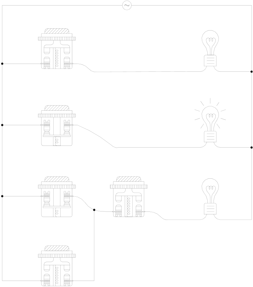
Actual wiring diagram
|
X0 X0 |
AC110V AC110V |
Y0 Y0 |
Circuit 1
NO(A) NO(A)
X1 X1 Y1 Y1
Circuit 2
|
NC(B) NC(B) |
X2 X2 |
X4 X4 |
Y2 Y2 |
Circuit 3
|
NC NC |
X3 X3 |
NO |
NO
NO
|
Conventional Ladder Diagram |
PLC Ladder Diagram |
||||||
|
circuit 1 |
X0 |
Y0 |
circuit 1 |
X0 |
X4 |
Y0 |
|
|
circuit 2 |
X1 |
Y1 |
circuit 2 |
X1 |
Y1 |
||
|
circuit 3 |
X2 |
X4 |
Y2 |
circuit 3 |
X2 |
Y2 |
|
|
X3 |
X3 |
||||||
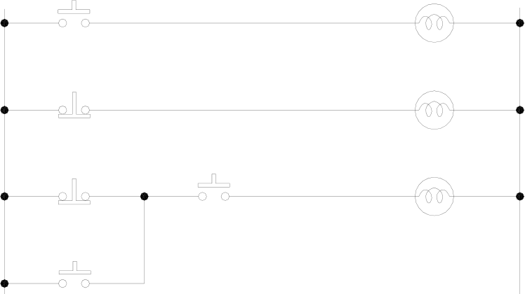
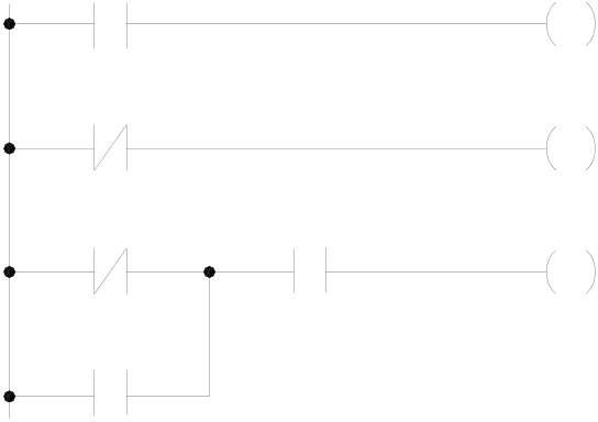
The above example illustrated the combination logic using the actual wiring diagram, conventional Ladder Diagram, and PLC Ladder Diagram. Circuit 1 uses a NO (Normally Open) switch that is also called "A" switch or contact. Under normal condition (switch is not pressed), the switch contact is at OFF state and the light is off. If the switch is pressed, the contact status turns ON and the light is on. In contrast, circuit 2 uses a NC (Normally Close) switch that is also called "B" switch or contact. Under normal condition, the switch contact is at ON state and the light is on. If the switch is pressed, the contact status turns OFF and the light also turns off.
Circuit 3 contains more than one input element. Output Y2 light will turn on under the condition when X2 is closed or X3 switches to ON, and X4 must switch ON too.
1.1.2Sequential Logic
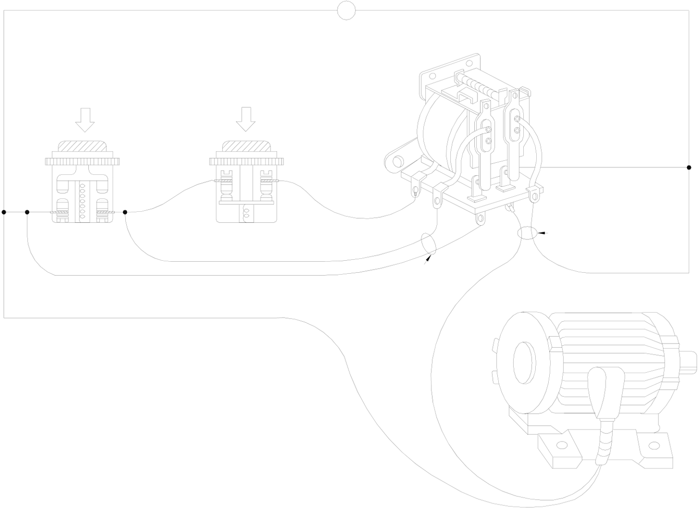
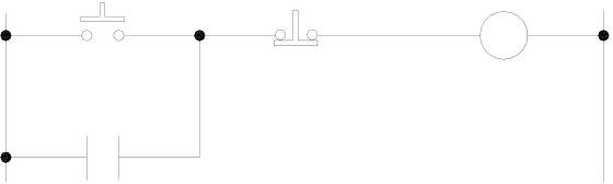
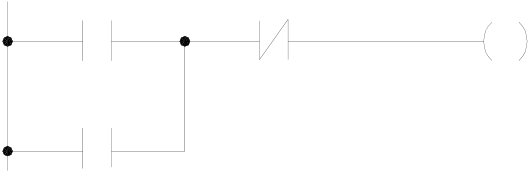
The sequential logic is a circuit with feedback control; that is, the output of the circuit will be feedback as an input to the same circuit. The output result remains in the same state even if the input condition changes to the original position. This
|
process can be best explained by the ON/OFF circuit of a latched motor driver as shown in below. Actual wiring diagram AC110V
Contact 1 Motor |
|
Conventional Ladder Diagram
|
PLC Ladder Diagram
|
||||||||
|
When we first connect this circuit to the power source, X6 switch is ON but X5 switch is OFF, therefore the relay Y3 is OFF. |
|||||||||
The relay output contacts 1and 2 are OFF because they belong to A contact (ON when relay is ON). Motor does not run. If we press down the switch X5, the relay turns ON as well as contacts 1and 2 are ON and the Motor starts. Once the relay turns ON, if we release the X5 switch (turns OFF), relay can retain its state with the feedback support from contact 1 and it is called Latch Circuit. The following table shows the switching process of the example we have discussed above.
|
c |
|
From the above table we can see that under different stages of sequence, the results can be different even the input statuses are the same. For example, let’s take a look at stage c and stage e , X5 and X6 switches are both released, but the Motor is ON (running) at stage e and is OFF (stopped) at stage c . This sequential control with the feedback of the output to the input is a unique characteristic of Ladder Diagram circuit. Sometimes we call the Ladder Diagram a "Sequential Control Circuit" and the PLC a "Sequencer”. In this section, we only use the A/B contacts and output coils as the example.
For more details on sequential instructions please refer to chapter 5 – "Introduction to Sequential Instructions."
1.2Differences Between Conventional and PLC Ladder Diagram
Although the basic operation principle for both conventional and PLC Ladder Diagram are the same, but in reality, PLC uses the CPU to emulate the conventional Ladder Diagram operations; that is, PLC uses scanning method to monitor the statuses of input elements and output coils, then uses the Ladder Diagram program to emulate the results which are the same as the results produced by the conventional Ladder Diagram logic operations. There is only one CPU, so the PLC has to sequentially examine and execute the program from its first step to the last step, then returns to the first step again and repeats the operation (cyclic execution). The duration of a single cycle of this operation is called the scan time. The scan time varies with the program size. If the scan time is too long, then input and output delay will occur. Longer delay time may cause big problems in controlling fast response systems. At this time, PLCs with short scan time are required. Therefore, scan time is an important specification for PLCs. Due to the advance in microcomputer and ASIC technologies nowadays the scan speed has been enhanced a great deal. A typical FBE-PLC takes approximately 0.33 ms for IK steps of contact. The following diagram illustrates the scanning process of a PLC Ladder Diagram.
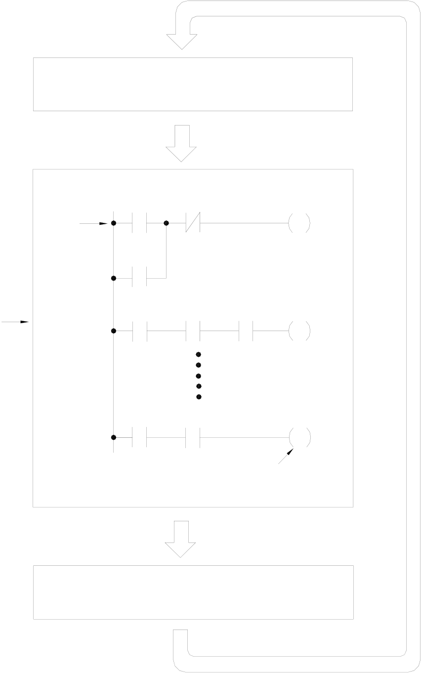
Input processing (Reading the
status of all external input terminals)
|
First |
X0 |
X1 |
Y0 |
step
Y0
|
PLC sequentially executes |
M100 |
X3 |
X10 |
Y1 |
Cyclic execution |
|
the stored program and |
|||||
|
gets new output results |
X100 |
M505 |
Y126 |
||
|
(has not sent to external |
|||||
|
terminals yet) |
Last step
Output processing (Output the resulting
signals to external output terminals)
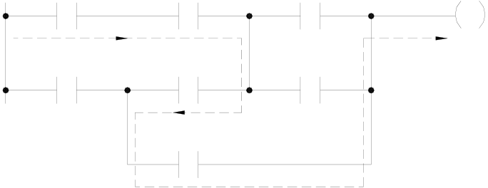
Besides the time scan difference mentioned above, the other difference between the conventional and PLC Ladder Diagram is “Reverse flow” characteristic. As shown in the diagram below, if X0, X1, X4 and X6 are ON, and the remaining elements are OFF. In a conventional Ladder Diagram circuit, a reverse flow route for output Y0 can be defined by the dashed line and Y0 will be ON. While for PLC, Y0 is OFF because the PLC Ladder Diagram scans from left to right, if X3 is off then CPU believes node “a” is OFF, although X4 and node “b” are all ON, since the PLC scan reaches X3 first. In other words, the PLC ladder can only allow left to right signal flow while conventional ladder can flow bi-directional.
Reverse flow of conventional Ladder diagram
|
X0 X0 |
a a |
X1 X1 |
b |
X2 X2 |
Y0 Y0 |
|
X3 X3 |
X4 X4 |
X5 X5 |
X6
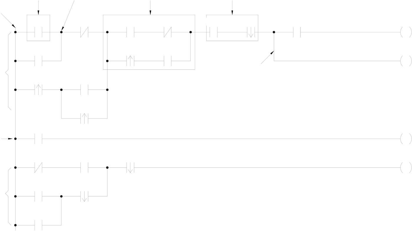
1.3Ladder Diagram Structure and Terminology
Sample Ladder Diagram
|
Element |
Node |
Parallel block |
Serial block |
Origin line
|
Network 1 |
X0 |
X1 |
X2 |
X3 |
X4 |
X5 |
X6 X6 |
Y0 |
|
X7 |
X11 |
X10 |
X9 |
Branch |
Y2 Y2 |
|||
|
/ |
||||||||
|
X10 |
Y4
X12 Y4
Network 2
|
M1 |
X14 |
X20 |
Y5 Y5 |
/
|
Network 3 |
Y0 |
M6 |
X16
(Remark:The maximum size of FBs-PLC network is 16 rows×22 columns)
As shown above, the Ladder Diagram can be divided into many small cells. There are total 88 cells (8 rows X 11 columns)
for this example Ladder Diagram. One cell can accommodate one element. A completed Ladder Diagram can be formed by
|
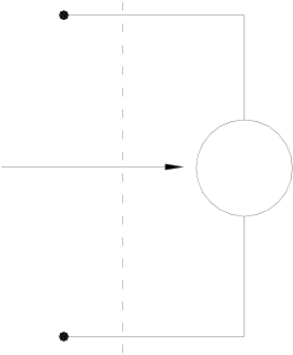
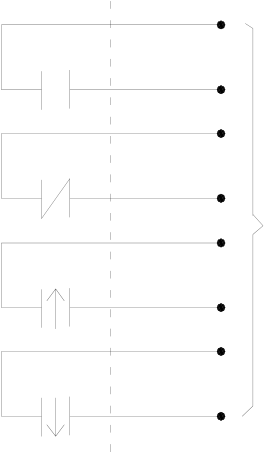
connecting all the cells together according to the specific requiremen illustrated below. c Contact Contact is an element with open or short status. One kind of contact is and its status reference from the external signals (the input signal c called "Relay contact" and its status reflects the status of relay coil (pl number and the contact status depends on the contact type. The con contact, B contact, up/down differential (TU/TD) contacts and Open/S d Relay Same as the conventional relay, it consists of a Coil and a Contact as
Y0 |
ts. The terminologies related to Ladder Diagram are called "Input contact"(reference number prefix with X) omes from the input terminal block). Another one is ease refer to d). The relation between the reference tact elements provided by FB series PLC include: A hort contacts. Please refer to f for more details. shown in the diagram below. TD |


|
Relay coil |
COIL |
Y0 |
A |
Relay contacts |
|
Y0 |
B |
|||
|
Y0 |
TU |
We must energize the coil of relay first (using OUT instruction) in order to turn on the relay. After the coil is energized, its contact status will be ON too. As shown in the example above, if Y0 turns ON, then the relay contact A is ON and contact B is OFF, TU contact only turns ON for one scan duration and TD contact is OFF. If Y0 turns OFF, then the relay contact A is ON and contact B is ON, TU contact is OFF and TD contact only turns ON for one scan duration (Please refer to chapter 4 “Introduction to Sequential Instructions” for operations of A,B,TU and TD contacts).
There are four types of FB-PLC relays, namely Y△△△(output relay), M△△△△(internal relay), S△△△(step relay)and TR△△(temporary relay). The statuses of output relays will be sent to the output terminal block.
e Origin-line: The starting line at the left side of the Ladder Diagram.
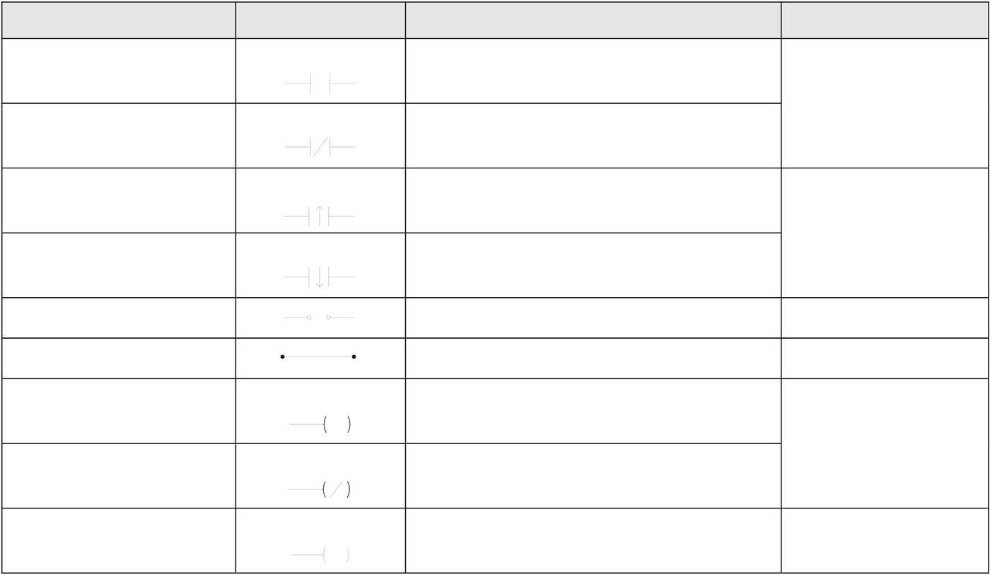
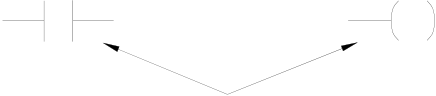
f Element: Element is the basic unit of a Ladder Diagram. An element consists of two parts as shown in the diagram below. One is the element symbol which is called “OP Code” and another is the reference number part which is called “Operand”.
Operand
|
X100 |
|
Y15 |
OP Code
|
Element type |
Symbol |
Mnemonic instructions |
Remark |
|
A Contact |
□△△△△ |
(ORG、LD、AND、OR) □△△△△ |
□ can be X、Y、M、S、 |
|
(Normally OPEN) |
|||
|
B Contact |
□△△△△ |
(ORG、LD、AND、OR) NOT |
T、C(please refer to |
|
section 2.2) |
|||
|
(Normally CLOSE) |
□△△△△ |
||
|
Up Differential Contact |
□△△△△ |
(ORG、LD、AND、OR) TU |
□ can be X、Y、M、S |
|
□△△△△ |
|||
|
Down Differential Contact |
□△△△△ |
(ORG、LD、AND、OR) TD |
|
|
□△△△△ |
□△△△△ |
||
|
Open Circuit Contact |
|||
|
(ORG、LD、AND、OR) OPEN |
|||
|
Short Circuit Contact |
(ORG、LD、AND、OR) SHORT |
||
|
Output Coil |
OUT □△△△△ |
□ can be Y、M、S
|
Inverse Output Coil |
□△△△△ |
OUT NOT □△△△△ |
|
Latching Output Coil |
Y△△△ |
OUT L Y△△△ |
|
L |
Remark:please refer to section 2.2 for the ranges of X、Y、M、S、T and C contacts. Please refer to section 4.2 for the characteristics of X、Y、M、S、T and C contacts.
There are three special sequential instructions, namely OUT TRn, LD TRn and FOn, which were not displayed on the Ladder Diagram. Please refer to section 1.6 “Using the Temporary Relay” and section 5.1.4 “Function Output FO”.
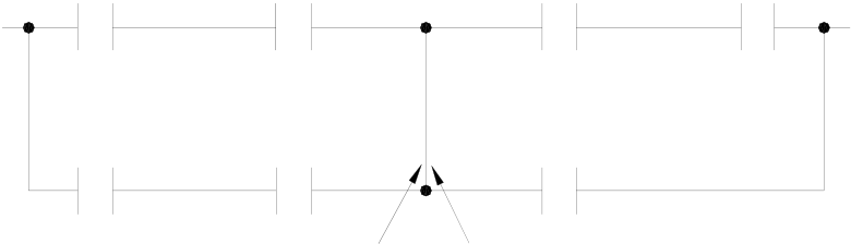
g Node: The connection point between two or more elements(please refer to section 4.3)
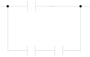
h Block: a circuit consists of two or more elements.
There are two basic types of blocks:
•Serial block:Two or more elements are connected in series to form a single row circuit.
Example: 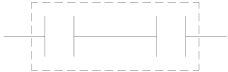
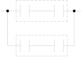
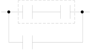
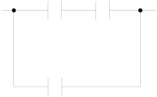
•Parallel block: Parallel block is a type of a parallel closed circuit formed by connecting elements or serial blocks in parallel.
|
Example: |
|
|
|
|
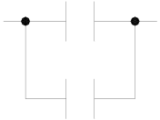
|
Remark: Complicated block can be formed by the combination of the single element, serial blocks and parallel blocks. When design a Ladder Diagram with mnemonic entry, it is necessary to break down the circuits into element, serial, and parallel blocks. Please refer to section 1.5. |
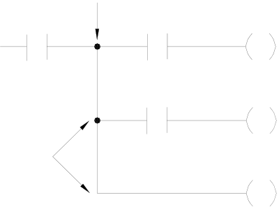
i Branch: In any network, branch is obtained if the right side of a vertical line is connected with two or more rows of circuits.
|
Example: |
|
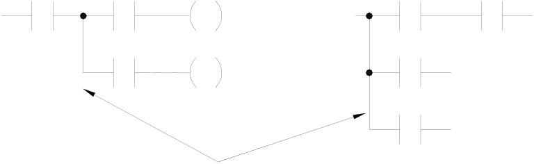
Branch
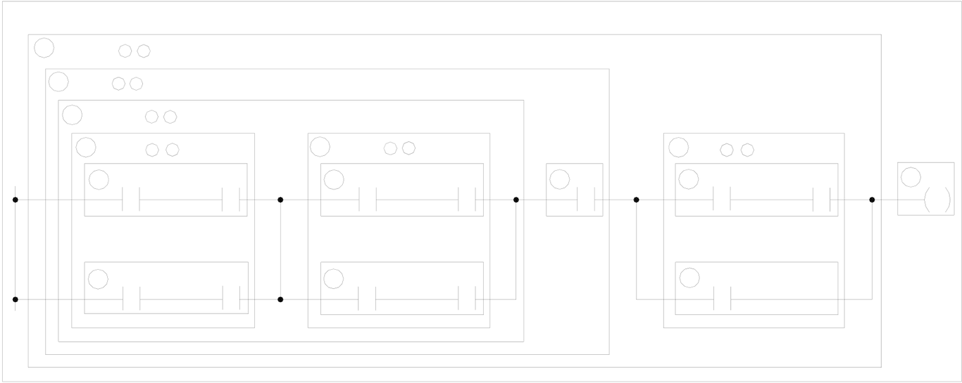
Merge line is defined as another vertical line at the right side of a branch line that merges the branch circuits into a closed circuit (forming a parallel block). This vertical line is called “Merge line”.
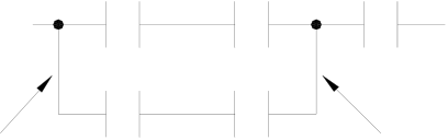
Branch lineMerge line
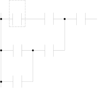
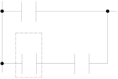
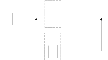
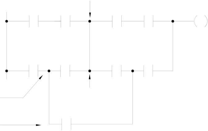
If both the right and the left sides of the vertical line are connected with two or more rows of circuits, then it is both a branch line and a merge line as shown in the example below.
Example:
Parallel block 1 Parallel block 2
Block 1 merge lineBlock 2 branch line

j Network: Network is a circuit representing a specified function. It consists of the elements, branches, and blocks. Network is the basic unit in the Ladder Diagram which is capable of executing the completed functions, and the program of Ladder Diagram is formed by connecting networks together. The beginning of the network is the origin line. If two circuits are connected by a vertical line, then they belong to the same network. If there is no vertical line between the two circuits, then they belong to two different networks. Figure 1, shows three (1~3) networks.
|
1.4The Coding Rules of Mnemonic |
(Users of WinProladder can skip this section) |
It’s very easy to program FB-PLC with WinProladder software package, just key-in the ladder symbols as they appear on your CRT screen directly to form a ladder diagram program. But for the users who are using FP-08 to program FB-PLC they have to translate ladder diagram into Mnemonic instructions by themselves. Since FP-08 only can input program with Mnemonic instruction, this section till section 1.6 will furnish you with the coding rules to translate ladder diagrams into Mnemonic instructions.
z The program editing directions are from left to right and from top to bottom. Therefore the beginning point of the network must be at the upper left corner of the network. Except the function instruction without the input control, the first instruction of a network must begin with the ORG and only one ORG instruction is permissible per network. Please refer to section 5.1.1 for further explanations.
|
Example: |
X0 |
X1 |
X5 |
Ö |
ORG |
X |
0 |
|
AND |
X |
1 |
|||||
|
X2 |
X4 |
||||||
|
LD |
X |
2 |
|||||
|
X3 |
OR |
X |
3 |
||||
|
AND |
X |
4 |
ORLD
|
AND |
X |
5 |
z Using LD instruction for connecting vertical lines (origin line or branch line) except at the beginning of the network.
|
Example 1: |
M0 |
X1 |
Ö |
ORG |
M |
0 |
|
X0 |
||||||
|
LD |
X |
0 |
||||
|
AND |
X |
1 |
ORLD
|
Example 2: |
Y0 |
M0 |
M1 |
Ö |
AND |
Y |
0 |
|
LD |
M |
0 |
|||||
|
X0 |
X1 |
AND |
M |
1 |
|||
|
LD |
X |
0 |
|||||
|
AND |
X |
1 |
ORLD
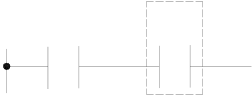
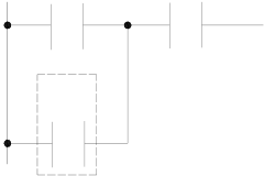
Remark 1: Using the AND instruction directly if only one row of elements is serially connected to the branch line.
|
Example: |
X0 |
Y0 |
Ö |
AND |
X |
0 |
|
ORLD |
Y |
0 |
||||
|
AND |

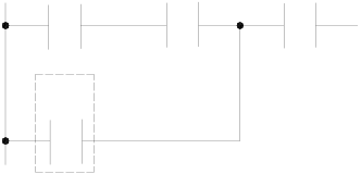
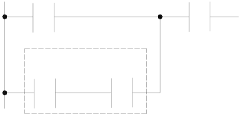
Remark 2: Also using the AND instruction directly if an OUT TR instruction has been used at a branch line to store the node statuses.
|
Example: |
OUT TR0 |
M0 |
X0 |
Y1 |
Ö |
AND |
M |
0 |
|
OUT TR |
0 |
|||||||
|
Y0 |
AND |
X |
0 |
|||||
|
OUT |
Y |
1 |
||||||
|
LD TR0 |
LDTR |
0 |
0 |
|||||
|
AND |
Y |
z Using AND instruction for serial connection of a single element.
|
Example: |
X0 |
X1 |
Ö |
ORG |
X |
0 |
|
AND |
X |
1 |
z Using OR instruction for parallel connection of a single element.
|
Example: |
X0 |
X2 |
X3 |
Ö |
ORG |
X |
0 |
|
OR |
X |
1 |
|||||
|
X1 |
|||||||
|
AND |
X |
2 |
|||||
|
Example: |
X0 |
X1 |
Ö |
ORG |
X |
0 |
|
|
AND |
X |
1 |
|||||
|
X2 |
OR |
X |
2 |
||||
|
AND |
X |
3 |
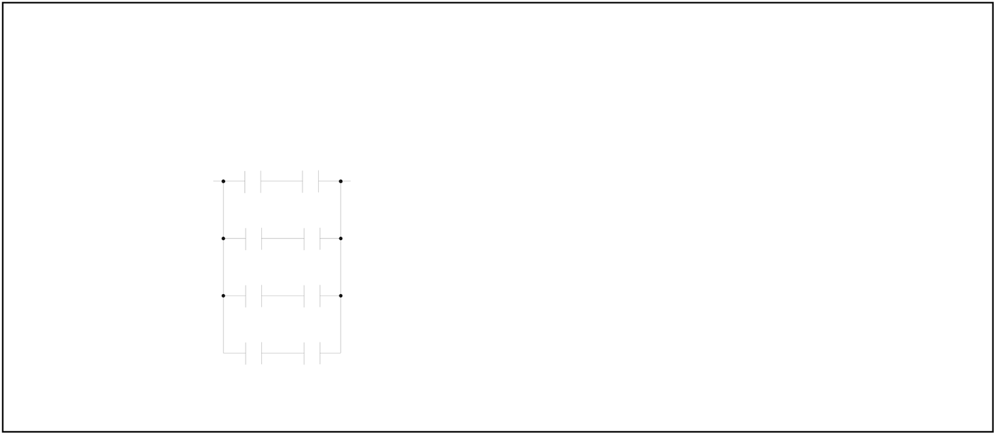
z If the parallel element is a serial block, ORLD instruction must be used.
|
Example: |
X2 |
X1 |
X3 |
Ö |
ORG |
X |
2 |
|
X0 |
LD |
X |
0 |
||||
|
AND |
X |
1 |
|||||
|
ORLD |
X |
3 |
|||||
|
AND |
Remark:If more than two blocks are to be connected in parallel, they should be connected in a top to bottom sequence. For example, block 1 and block 2 should be connected first, then connect block 3 to it and so on.
|
Example: |
X0 |
M0 |
Ö |
LD |
X |
0 |
|
AND |
M |
0 |
||||
|
X1 |
M1 |
LD |
X |
1 |
||
|
AND |
M |
1 |
||||
|
X2 |
M2 |
ORLD |
X |
2 |
||
|
LD |
||||||
|
X3 |
M3 |
AND |
M |
2 |
||
|
ORLD |
X |
3 |
||||
|
LD |
||||||
|
AND |
M |
3 |
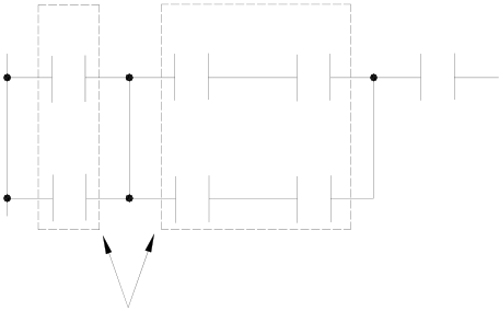
z ANDLD instruction is used to connect parallel blocks in series.
|
Example: |
X1 |
X3 |
X4 |
X7 |
Ö |
ORG |
X |
1 |
|
OR |
X |
2 |
||||||
|
LD |
X |
3 |
||||||
|
X2 |
X5 |
X6 |
AND |
X |
4 |
|||
|
LD |
X |
5 |
||||||
|
AND |
X |
6 |
ORLD
|
Must use ANDLD instruction |
ANDLD |
X |
7 |
|
AND |
z The ANDLD instruction must be used if the element or serial block is in front of the parallel block. If the parallel block is in front of the element or serial block, AND instruction can be used to connect all parts together.
|
Example: |
Serial Block |
ANDLD instruction |
Ö |
ORG |
X |
0 |
||
|
is not necessary |
AND |
X |
1 |
|||||
|
X2 |
X4 |
LD |
X |
2 |
||||
|
X0 |
X1 |
|||||||
|
OR |
X |
3 |
||||||
|
X3 |
ANDLD |
X |
4 |
|||||
|
AND |
||||||||
Must use ANDLD instruction
|
Remark: If there are more than two blocks are to be connected serially, they should be connected in a top to bottom sequence. For example, block 1 and 2 should be connected first, then connect block 3 to it and so on.
ANDLD |
z The output coil instruction (OUT)can only be located at end of the network (the right end) and no other elements can be connected to it afterwards. The output coil can not connect to the origin line directly. If you want to connect the output coil to the origin line, connect it serially with a short circuit contact.
|
Y0 |
Ö |
ORG SHORT |
Y |
0 |
|
|
OUT |

|
1.5The De-Composition of a Network(Users of WinProladder can skip this section) |
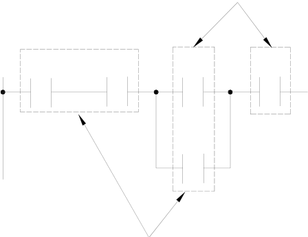
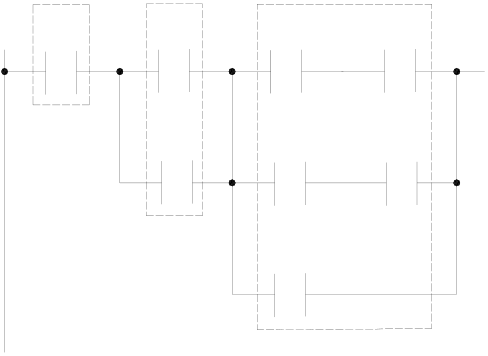
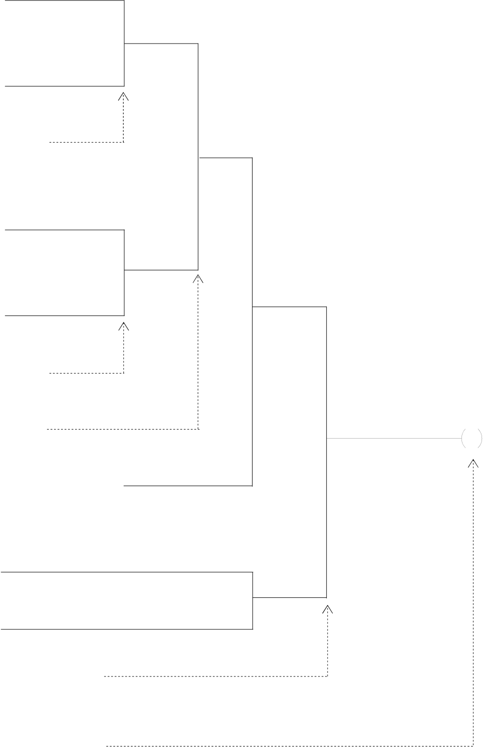
The key process of de-composition of a network is to separate the circuits that appear between two vertical lines into independent elements and serial blocks, then coding those elements and serial blocks according to the mnemonic coding rules and then connect them (with ANDLD or ORLD instruction) from left to right and top to bottom to form a parallel or a serial-parallel blocks, and finally to form a complete network.
Sample diagram:
|
13 |
ANDLD( ) |
6 |
ORLD( ) |
X5 |
8 |
X8 |
12 |
OR( ) |
X10 |
14 |
Y0 |
|||||
|
9 |
||||||||||||||||
|
AND( ) |
||||||||||||||||
|
7 |
ANDLD( ) |
|||||||||||||||
|
3 |
ORLD( ) |
|||||||||||||||
|
1 |
X0 |
X1 |
4 |
X4 |
10 |
X9 |
||||||||||
|
ORG |
X3 |
X7 |
||||||||||||||
|
2 |
X2 |
5 |
X6 |
11 |
X11 |
|||||||||||
|
X0 |
|
|||||||||||||||
|
Serial blockc |
||||||||||||||||
|
AND |
||||||||||||||||
e
|
LD |
X2 |
|
Serial blockd |
i |
|
|
AND |
X3 |
||||
|
ORLD |
Forming the parallel |
||||
|
X4 |
|
||||
|
LD |
block e |
||||
|
Serial blockf |
|||||
|
AND |
X5 |
h
|
LD |
X6 |
|
Serial blockg |
k |
|||
|
AND |
X7 |
||||||
|
ORLD |
Forming the parallel |
||||||
|
X8 |
|
○ |
○ |
Y0 Y0 |
|||
|
ANDLD |
block h |
||||||
|
Forming the serial |
|||||||
|
block i |
|||||||
|
AND |
|||||||
|
Serial blockiAND element j |
|||||||
|
LD |
X9 |
Serial block ○ |
|||||
|
AND |
X10 |
||||||
|
OR |
X11 |
OR element ○ |
|||||
|
Forming the serial block ○ |
|||||||
|
Y0 |
|||||||
|
OUT |
Send the ○13result to Y0 |
|
1.6Using Temporary Relays (Users of WinProladder can skip this section) |
The network de-composition method for mnemonic coding demonstrated in section 1.5 does not apply to the branched circuit or branched block. In order to input the program using the method shown in section 1.5, It must first to store the statuses of branched nodes in temporary relays. The program design should avoid having branched circuit or branched block as much as possible. Please refer the next section “Program Simplification Techniques”. Two situations that must use the TR are described at below.
z Branched circuit: Merge line does not exist at the right side of the branch line or there is a merge line at the right side of the branch line but they are not in the same row.
Example: * indicates setting of TR relay
Without merge line
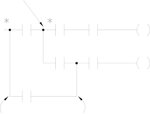
Although this branch has merge lines
but they are not in the same row, so this
is also a branched circuit
z Branched block:The horizontal parallel blocks with a branch in one of the blocks.
Example: Merge line
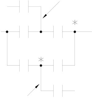
Branch line
|
Remark 1: The OUT TR instruction must be programmed at the top of the branched point. LD TRn instruction is used at the starting point of the circuits after second rows of the branch line for regaining the branch line status before you can connect any element to the circuits. AND instruction must be used to connect the first element after OUT TRn or LD TRn instruction. LD instruction is not allowed in this case. Remark 2: A network can have up to 40 TR points and the TR number can not be used repeatedly in the same network. It is recommended to use the numbers 1,2,3… with sequence. The TR number must be the same in the same branch line. For example, if a branch line uses OUT TR0, then starting from row 2, LD TR0 must be used for connection. Remark 3: If the branch line of a branched circuit or a branched block is the origin line, then ORG or LD instructions can be used directly and TR contact is not necessary. Remark 4: If any one of the branched circuit rows is not connected to the output coil (there are serially connected elements in between), and other circuits also exist after the second row, a TR instruction must be used at the branch points. |
|
Example: |
OUT TR0 |
Y0 |
Y0 |
Ö |
AND |
X |
0 |
|||||||
|
OUT TR |
0 |
1 |
||||||||||||
|
X0 |
X1 |
AND |
X |
|||||||||||
|
OUT |
Y |
0 |
||||||||||||
|
X2 |
Y1 |
|||||||||||||
|
LD TR |
0 |
←─ Begins from row 2 |
||||||||||||
|
Example: |
LD TR0 |
Y2 |
Ö |
AND |
X |
2 |
||||||||
|
OUT |
Y |
1 |
||||||||||||
|
LD TR |
0 |
←─ Begins from row 3 |
||||||||||||
|
OUT |
Y |
2 |
||||||||||||
|
OUT TR1 |
||||||||||||||
|
ORG |
X |
1 |
||||||||||||
|
AND |
X |
2 |
||||||||||||
|
* |
LD |
X |
3 |
|||||||||||
|
X1 |
X2 |
X5 |
X6 |
|||||||||||
|
OUTTR |
0 |
|||||||||||||
|
block 1 |
block 2 |
AND |
X |
4 |
||||||||||
|
X3 |
X4 |
X7 |
X8 |
ORLD |
||||||||||
|
OUT TR0 |
1 |
|||||||||||||
|
OUTTR |
5←─ Uses AND Instruction 6 after TR instruction |
|||||||||||||
|
LD TR1 |
||||||||||||||
|
AND |
X |
|||||||||||||
|
X9 |
block 3 |
AND |
X |
|||||||||||
|
LD TR0 |
||||||||||||||
|
7 |
←─ |
Uses LD TR instruction to return to TR branch line |
||||||||||||
|
LD TR |
1 |
|||||||||||||
|
AND |
X |
|||||||||||||
|
LD TR |
0 |
9←─ Uses AND instruction after TR instruction |
||||||||||||
|
AND |
X |
|||||||||||||
|
ORLD |
||||||||||||||
|
AND |
X |
8 |
||||||||||||
ORLD
|
OUT |
Y |
0 |
z The above sample diagram shows a typical example of connecting two parallel blocks in series. Block 3 is formed when
the element X9 is introduced into the network and the two parallel blocks become the branched blocks.
z TR instruction is not necessary because the(*)point is the origin line.
z If have already used TR relay to connect two blocks serially, then ANDLD instruction is not necessary.
1.7Program Simplification Techniques
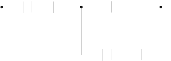
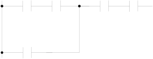
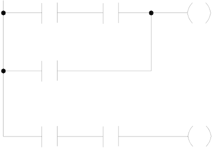
z If a single element is connected in parallel to a serial block, The ORLD instruction can be omitted if the serial block is
connected on top of this single element.
|
LD |
X0 |
X |
X2 |
0 |
Ö |
X1 |
X2 |
X |
1 |
|
X1 |
X0 |
LD |
|||||||
|
LD |
X |
1 |
AND |
X |
2 |
||||
|
AND |
X |
2 |
OR |
X |
0 |
ORLD
z When a single element or a serial block is connected in serial with a parallel block, ANDLD instruction can be omitted if put the parallel block in front.
|
X0 |
X1 |
X2 |
X4 |
Ö |
X3 |
X4 |
X |
3 |
X0 |
X1 |
|
X3 |
X2 |
|||||||||
|
ORG |
X |
0 |
ORG |
|||||||
|
AND |
X |
1 |
AND |
X |
4 |
|||||
|
LD |
X |
2 |
OR |
X |
2 |
|||||
|
LD |
X |
3 |
AND |
X |
0 |
|||||
|
AND |
X |
4 |
AND |
X |
1 |
ORLD
ANDLD
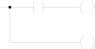
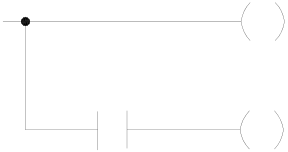
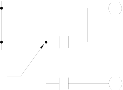
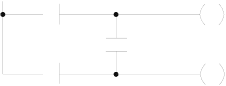
z If the branch node of a branch circuit is directly connected to the output coil, this coil could be located on top of the branch line (first row) to reduce the code.
|
X0 |
0 |
Y0 |
Ö |
X0 |
Y |
Y1 |
1 |
|
OUT TR |
Y1 |
Y0 |
|||||
|
OUT |
|||||||
|
AND |
X |
0 |
AND |
X |
0 |
||
|
OUT |
Y |
0 |
OUT |
Y |
0 |
||
|
LDTR |
0 |
1 |
|||||
|
OUT |
Y |
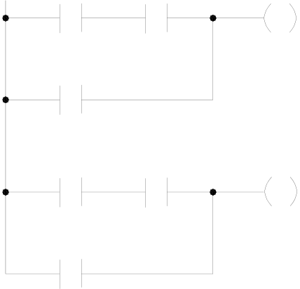
z The diagram shown below indicates the TR relay and the ORLD instruction can be omitted.
|
X0 |
X2 |
0 |
Y0 |
Ö |
ORG |
X1 |
X2 |
Y0 |
|
X1 |
X0 |
|||||||
|
OUT TR0 |
X3 |
Y1 |
X1 |
X3 |
Y1 |
|||
|
ORG |
X |
X |
1 |
|||||
|
LD |
X |
1 |
AND |
X |
2 |
|||
|
OUT TR |
0 |
2 |
OR |
X |
0 |
|||
|
AND |
X |
OUT |
Y |
0 |
||||
|
ORLD |
Y |
0 |
ORG |
X |
1 |
|||
|
OUT |
AND |
X |
3 |
|||||
|
LDTR |
0 |
3 |
OUT |
Y |
1 |
|||
|
AND |
X |
|||||||
|
OUT |
Y |
1 |
z Conversion of the bridge circuit
|
X0 |
Y0 |
Ö |
X1 |
X2 |
1 |
Y0 |
|
|
X1 |
X2 |
Y1 |
X0 |
X2 |
Y1 |
||
|
X0 |
|||||||
|
This network structure is not |
X1 |
X |
|||||
|
allowed in PLC program |
|||||||
|
ORG |
|||||||
|
AND |
X |
2 |
|||||
|
OR |
X |
0 |
|||||
|
OUT |
Y |
0 |
|||||
|
ORG |
X |
0 |
|||||
|
AND |
X |
2 |
|||||
|
OR |
X |
1 |
|||||
|
OUT |
Y |
1 |
|||||
Tip: press ← → to switch chapters, Ctrl+K to search